My Executive Summary on Quantum Computing
Quick take: Quantum computing matters because it expands what problems are feasible, not just how fast we solve them.
In this summary
- Why raw computation powers modern life
- Where classical computing hits hard limits (P vs NP)
- What makes qubits different
- Why quantum hardware is so hard to build
Contents
- Why We Care
- Classical Computing in One Idea
- Where Classical Hits Limits
- Classical Bits Versus Quantum Bits
- So Why Is This So Hard to Build?
- Where We Are Today
- Key takeaways
Why We Care
A simple question with a surprisingly deep answer.
Take a moment and ask yourself a few simple questions:
- How did your phone know the fastest route to get you home today?
- How can Netflix predict what you want to watch next?
- How does your laptop recognize your face, compress video, or render a 3D game in real time?
- How does your bank detect fraud in milliseconds?
All of these feel ordinary now. None of them are simple.
Behind every one of these conveniences is an enormous amount of computation. Trillions of tiny operations are happening every second. At their core, all of this complexity reduces to an almost laughably simple idea: strings of 0s and 1s being manipulated at extreme speed.
Modern computers are not intelligent in the human sense. They do not understand images, language, or meaning. They are extremely fast machines for performing logical operations on binary data. The reason our digital world feels intelligent is not because the problems are easy, but because our processors are powerful enough to brute force solutions that would have been impossible just a few decades ago.
Without that computational power:
- GPS navigation would not exist
- Real time video calls would be impossible
- Weather prediction would be wildly inaccurate
- Medical imaging and protein modeling would be severely limited
- Modern cryptography would not work
In short, much of modern life quietly depends on raw computational horsepower.
The key idea
Every major leap in computing power unlocks entirely new categories of technology.
Quantum computing sits on the edge of that same kind of transition.
Every major leap in computing power has unlocked entirely new categories of technology. Not just faster versions of old tools, but things people did not even know to ask for. Before classical computers, no one imagined search engines, real time translation, or machine learning. Those ideas only became possible after the hardware existed.
Quantum computing sits at the edge of that same kind of transition.
It does not replace classical computers, just as airplanes did not replace cars. Instead, it offers a fundamentally different way of processing information, one that can outperform classical machines for certain types of problems.
And just like someone in the 1950s could not have predicted smartphones, we likely do not yet have the language to describe the most important applications of quantum computing.
That is why we care.
Not because quantum computers are simply faster, but because they may allow us to ask questions, solve problems, and build technologies that are currently beyond the limits of classical computation.
Takeaway: Quantum computing is about new capability, not just raw speed.
Classical computing in one idea
At the most fundamental level, a classical computer works with bits.
A bit can be in exactly one of two states:
That is it. No hidden complexity. No extra options.
At first glance, this seems incredibly limiting. How could anything interesting come from just two values?
The answer is that combinations of bits scale extremely fast.
Rule of thumb: each additional bit doubles the number of representable values.
From bits to numbers
With a single bit, you can represent two values.
With two bits, you can represent four.
With three bits, eight.
With four bits, sixteen.
Here is what that looks like in practice:
| Binary | Base 10 |
|---|---|
| 000 | 0 |
| 001 | 1 |
| 010 | 2 |
| 011 | 3 |
| 100 | 4 |
| 101 | 5 |
| 110 | 6 |
| 111 | 7 |
Just three bits already give you eight distinct values.
A modern 64 bit computer can represent:
different numbers.
That is more than enough to index memory, represent timestamps, encode colors, store images, and perform scientific calculations.
From numbers to everything else
Once you can represent numbers, everything else follows.
Text is just numbers mapped to letters.
| Character | Binary |
|---|---|
| A | 01000001 |
| B | 01000010 |
| C | 01000011 |
Images are grids of numbers representing color intensities.
Audio is a sequence of numbers representing air pressure over time.
Video is just many images shown quickly.
Even something as abstract as a neural network reduces to:
- numbers stored in memory
- multiplications and additions
- repeated millions or billions of times
There is no magic. Just arithmetic performed extremely fast.
How arithmetic actually works in binary
Okay so if everything is arithmetic, then how does that work?
Let us start with something familiar.
Binary addition
Here is what addition looks like in base 10:
Now the same idea in binary:
  0111   (7)
+ 0101   (5)
-------
  1100   (12)
The rules are exactly what you would expect:
- 0 + 0 = 0
- 0 + 1 = 1
- 1 + 0 = 1
- 1 + 1 = 0, carry the 1
That carry operation is the key. It is how addition scales from a single bit to arbitrarily large numbers.
A processor performs this using logic gates. No numbers in the human sense. Just voltage levels representing 0 or 1.
Multiplication is just repeated addition
Now take multiplication.
In binary:
0110   (6)
×
0011   (3)
=
0110
+
0110
+
0110
=
10010   (18)
This is exactly the same process you learned in school, just expressed in base 2.
A computer does not know it is multiplying. It just applies bit shifts and additions extremely fast.
How this becomes images and video
Once you accept that numbers are easy, everything else follows naturally.
An image is just a grid of numbers.
For example, a grayscale pixel might look like this:
| Value | Brightness |
|---|---|
| 0 | Black |
| 128 | Gray |
| 255 | White |
A color image simply uses three numbers per pixel:
- Red intensity
- Green intensity
- Blue intensity
A video is just many of these images shown in rapid succession.
Audio works the same way. The computer stores how much air pressure should exist at each moment in time and plays it back quickly enough that your ear perceives a continuous sound.
At no point does the computer see a face, hear a voice, or understand a song.
It only ever sees numbers.
The important takeaway
Every modern digital experience is built on:
- Binary numbers
- Simple arithmetic
- Massive repetition
- Extreme speed
That is the entire trick.
And it works unbelievably well.
But it also reveals the limitation.
When problems become too large, too complex, or too interconnected, the number of operations required grows faster than classical computers can handle.
That is not a software problem.
That is a fundamental limit of how classical computation works.
And that is exactly the gap quantum computing is designed to explore.
Where Classical Hits Limits
Why classical scales
The real power of classical computing is not that the rules are clever.
It is that the rules are simple enough to scale.
Modern processors can perform billions of operations per second. When you combine that speed with decades of engineering, you get:
- Real time graphics
- Speech recognition
- GPS navigation
- Medical imaging
- Machine learning
All of it built on nothing more than 0s and 1s.
And now the limitation
Here is the catch.
Some problems grow so fast that even the best classical computers cannot keep up.
Not because engineers failed.
Not because we need better code.
But because the number of possibilities explodes faster than classical hardware can handle.
This is not an engineering problem.
It is a mathematical one.
When fast is not fast enough
Up until now, everything we have talked about works because computers can do a lot of simple operations very quickly. But what if a lot is still not enough?
Let me show you what I mean.
Suppose I ask you to list every possible ordering of the four aces in a deck of cards.
That sounds easy. There are only four cards.
Example: factorial explosion
Even for 4 items, the number of arrangements grows quickly.
Here is the full list:
- {Spade, Heart, Diamond, Club}
- {Spade, Heart, Club, Diamond}
- {Spade, Diamond, Heart, Club}
- {Spade, Diamond, Club, Heart}
- {Spade, Club, Heart, Diamond}
- {Spade, Club, Diamond, Heart}
- {Heart, Spade, Diamond, Club}
- {Heart, Spade, Club, Diamond}
- {Heart, Diamond, Spade, Club}
- {Heart, Diamond, Club, Spade}
- {Heart, Club, Spade, Diamond}
- {Heart, Club, Diamond, Spade}
- {Diamond, Spade, Heart, Club}
- {Diamond, Spade, Club, Heart}
- {Diamond, Heart, Spade, Club}
- {Diamond, Heart, Club, Spade}
- {Diamond, Club, Spade, Heart}
- {Diamond, Club, Heart, Spade}
- {Club, Spade, Heart, Diamond}
- {Club, Spade, Diamond, Heart}
- {Club, Heart, Spade, Diamond}
- {Club, Heart, Diamond, Spade}
- {Club, Diamond, Spade, Heart}
- {Club, Diamond, Heart, Spade}
That is already 24 possibilities from just 4 cards.
This happens because the number of possible arrangements grows as a factorial.
With 4 cards, there are:
With a full deck of 52 cards:
For comparison, there are only about:
atoms in the entire Earth.
There are more ways to arrange a deck of cards than there are atoms on the planet.
Clearly, no computer could ever list them all. Not because computers are slow, but because the number of possibilities explodes too fast.
Verification versus solving
Now consider a different kind of problem.
Imagine I hand you a completed Sudoku puzzle and ask:
“Is this solution valid?”
You can check it quickly. Scan the rows, columns, and boxes. Easy.
Now imagine I give you a blank Sudoku puzzle and ask you to solve it.
That task is much harder.
This distinction matters.
Checking a solution can be easy, even when finding the solution is extremely difficult.
This difference is at the heart of the P versus NP problem.
Key distinction: verifying a solution can be easy even when finding it is hard.
What P and NP actually mean
Computer scientists have names for these categories:
- P contains problems that can be solved efficiently
- NP contains problems whose solutions can be verified efficiently
The million dollar question is: if a solution can be verified quickly, can it also always be found quickly?
Most computer scientists believe the answer is no. There exist problems that are easy to check but fundamentally hard to solve.
Why this matters
If P were equal to NP, then problems like:
- Optimal scheduling
- Protein folding
- Route optimization
- Cryptographic cracking
would suddenly become easy.
But if P is not equal to NP, then some problems are hard not because we lack clever algorithms, but because the mathematics itself makes them hard.
No amount of hardware improvement would change that.
What this has to do with quantum computing
Quantum computers do not magically make P equal NP.
They do not turn every hard problem into an easy one.
But they do change something very important: the computational model itself.
P and NP describe what is hard or easy for classical computers. But quantum computers follow different rules. When you change the rules, some problems that looked hard can become easy.
This is exactly what quantum computing does.
Classical vs quantum complexity
In classical computing:
- P = problems solvable efficiently
- NP = problems whose solutions can be verified efficiently
In quantum computing, we introduce a new class:
- BQP = problems solvable efficiently on a quantum computer
These are not the same sets.
Quick glossary
| Term | Meaning (informal) |
|---|---|
| P | Problems that can be solved efficiently on a classical computer |
| NP | Problems whose solutions can be verified efficiently on a classical computer |
| BQP | Problems that can be solved efficiently on a quantum computer |
Some problems that appear hard for classical computers are believed to fall into BQP, meaning they are efficiently solvable on a quantum computer even though no efficient classical algorithm is known.
The most famous example is integer factorization.
Factoring large numbers:
- Is not known to be in classical P
- Is not believed to be NP-complete
- Is known to be in BQP, thanks to Shor's algorithm
From a classical perspective, factoring looks hard.
From a quantum perspective, it is efficiently solvable.
That does not mean quantum computers solve all NP problems.
It means that some problems that appear hard classically are not hard in the quantum model.
The important distinction
This is the key idea:
Complexity classes depend on the computational model.
A problem being “hard” in classical computing does not mean it is fundamentally hard in every possible model of computation.
Quantum computing does not collapse NP into P.
But it does redefine what “efficiently solvable” means for certain problems.
So when people say quantum computing has revolutionary potential, they do not mean it breaks mathematics.
They mean it operates under different rules (rules that allow some problems to move from "infeasible" to "tractable").
Why this matters for real problems
If a problem lies in:
- classical NP
- but quantum P (BQP)
then quantum computers can solve it efficiently even though classical computers likely never will.
That is an extraordinary shift.
It means the limits of classical computation are not the limits of computation itself.
And that is why quantum computing is interesting.
Not because it makes everything fast.
But because it changes which problems are fast at all.
Classical bits versus quantum bits
Up to this point, everything we have discussed has relied on a single assumption: a bit is either a 0 or a 1.
That assumption is so natural that it rarely gets questioned. But it is also the point where classical and quantum computing fundamentally diverge.
The classical bit
A classical bit can be in one of two states:
Nothing in between. No ambiguity.
At any moment in time, the bit has a definite value. Even if we do not know what it is, the value exists.
All classical computation is built on this idea.
The quantum bit
A quantum bit, or qubit, behaves very differently.
Instead of being restricted to just 0 or 1, a qubit can exist in a superposition of both.
Using bra-ket notation, we write this as:
Here:
- and are the quantum versions of classical 0 and 1
- and are complex numbers
- and give the probabilities of measuring 0 or 1
The only constraint is:
This means the qubit is not “partially 0 and partially 1” in a vague sense.
It exists in a precise mathematical combination of both.
Important note
You may be inclined to think that a qubit is actually always in either the or state, and that we simply do not know which one until we measure it. This intuition is incorrect.Before measurement, the qubit is not in the or state.
There is no hidden information we are missing. No additional knowledge we could obtain that would allow us to predict the outcome with certainty.
The only meaningful statement we can make is probabilistic:
The qubit will be measured as with probability ,
and as with probability .
Nothing more. Nothing less.
This is not a limitation of our measurement tools. It is a fundamental feature of quantum mechanics.
From two points to a continuous space
A classical bit lives at one of two points:
A qubit, however, lives on a continuous surface.
This is usually visualized using the Bloch sphere.
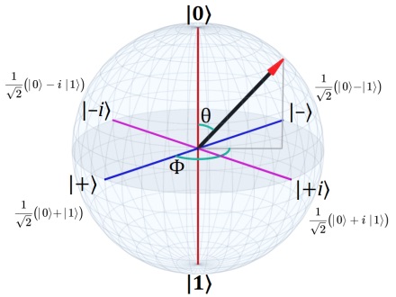 Bloch sphere visualization
Every possible pure qubit state corresponds to a point on the surface of a sphere.
- The north pole represents
- The south pole represents
- Every other point represents a superposition of the two
Instead of two discrete states, a qubit has an infinite continuum of possible states.
This is the first place where quantum computation begins to feel fundamentally different.
Why this matters
At first glance, this might seem like a small change.
After all, when you measure a qubit, you still only get a 0 or a 1.
But the power of quantum computing does not come from measurement.
It comes from what happens before measurement.
While a classical bit can only be in one state at a time, a qubit can evolve through an entire space of possibilities. When multiple qubits become entangled, the number of possible configurations grows exponentially.
Common misconception: “A quantum computer tries all answers at once.”
Reality: Quantum systems manipulate probability amplitudes. Through interference, some possibilities are amplified while others cancel out.
This is where quantum speedups come from.
A useful way to think about it
A classical bit is like a coin lying flat on a table.
It is either heads or tails.
A qubit is like a spinning coin.
While it is spinning, it is not heads or tails, but something in between. And how you choose to observe it determines what you see.
The Bloch sphere captures this idea visually.
And this continuous structure is where much of quantum computing's potential power originates.
Mental model: classical bit = coin on the table; qubit = spinning coin.
So why is this so hard to build?
If quantum computing offers such revolutionary potential, why are we not all using quantum laptops?
The answer comes down to a single brutal fact: quantum states are extraordinarily fragile.
Why it's hard, in brief
- Decoherence
- Temperature
- Errors
- Connectivity
- Scaling
- Algorithms
The problem of decoherence
Remember that a qubit exists in a superposition of states. This superposition is not just a mathematical abstraction. It is a physical reality that must be maintained long enough to perform useful computation.
But here is the catch: the moment a qubit interacts with its environment (air molecules, stray electromagnetic fields, even cosmic rays), it begins to lose its quantum properties. This process is called decoherence.
Classical bits do not have this problem. A bit stored in memory can sit there indefinitely. Even if the voltage fluctuates slightly, the bit remains a 0 or a 1. The system is robust to small perturbations.
Qubits are not.
A qubit's superposition is so delicate that even the slightest unintended interaction can destroy it. Once decoherence occurs, the qubit behaves like a classical bit, and all quantum advantage is lost.
Current quantum computers can maintain coherence for only milliseconds to seconds. That might sound like a lot, but quantum algorithms require thousands or millions of operations. If your qubits decohere before the algorithm finishes, the computation fails.
The temperature problem
To minimize decoherence, most quantum computers operate at temperatures close to absolute zero. We are talking about 0.015 Kelvin, which is colder than outer space.
Why?
At higher temperatures, thermal energy causes atoms to vibrate. These vibrations introduce noise that disrupts the fragile quantum states. Cooling the system to near absolute zero reduces this thermal noise to a minimum.
But maintaining these temperatures requires massive dilution refrigerators that cost hundreds of thousands of dollars and consume enormous amounts of energy. This is not something you can fit in a laptop.
The error problem
Even in perfect isolation at near absolute zero, quantum operations are not perfect. Every gate operation introduces a small amount of error. Over thousands of operations, these errors accumulate.
Classical computers solve this problem with error correcting codes. If a bit flips from 0 to 1 due to a cosmic ray, redundancy allows the system to detect and fix it.
Quantum error correction is much harder.
You cannot simply copy a qubit (thanks to the no-cloning theorem). And measuring a qubit to check for errors collapses its superposition, destroying the very information you are trying to protect.
The solution is quantum error correction, which encodes a single logical qubit across many physical qubits. If one physical qubit experiences an error, the redundancy allows the system to detect and correct it without collapsing the logical qubit.
But here is the problem: current quantum error correction codes require 100 to 1000 physical qubits to encode a single logical qubit. This means a useful quantum computer with 1000 logical qubits might require 100,000 to 1,000,000 physical qubits.
Today's largest quantum computers have only a few thousand physical qubits. And many of those qubits are too noisy to be useful.
The connectivity problem
In classical computers, any piece of data can interact with any other piece of data through memory and buses. Connectivity is not a fundamental constraint.
In quantum computers, qubits must be physically connected to interact. Two qubits that are not directly connected cannot perform a two-qubit gate without routing the operation through intermediate qubits. This routing introduces additional operations, which introduces more errors, which makes the problem worse.
Most current quantum computers have limited connectivity. Each qubit can only interact with a few neighbors. This architectural constraint makes it harder to implement algorithms efficiently.
The scaling problem
Even if we solve decoherence, error correction, and connectivity, there is still the question of scale.
A truly useful quantum computer (one that can outperform classical computers on real world problems) will likely need millions of high-quality qubits. Building systems at that scale introduces engineering challenges that dwarf anything we have solved so far.
Cooling systems, control electronics, wiring, calibration, and synchronization all become exponentially harder as the number of qubits grows.
The algorithm problem
Finally, even if we build a perfect quantum computer, we still need algorithms that actually use it well.
Quantum algorithms are not like classical algorithms. They require a completely different way of thinking. And for many problems, we simply do not know if a quantum speedup is even possible.
Shor's algorithm (for factoring) and Grover's algorithm (for search) are famous because they are among the few examples where we know quantum computers have a clear advantage. But there are entire categories of problems where it is still an open question whether quantum computing helps at all.
Where we are today
Despite all these challenges, progress is accelerating.
Companies like IBM, Google, and IonQ are building quantum computers with hundreds of qubits. Error rates are improving. New error correction techniques are being developed. And researchers are discovering new algorithms.
We are not at the point where quantum computers are practical for most problems. But we are past the point where they are purely theoretical.
The most likely path forward is hybrid systems: classical computers handle most of the work, and quantum computers tackle specific subroutines where they have an advantage.
Over time, as hardware improves and error correction becomes more efficient, the range of problems that benefit from quantum computing will expand.
But for now, quantum computing remains one of the hardest engineering challenges humanity has ever attempted.
The physics works. The math works. The algorithms exist.
The challenge is building machines that can actually run them reliably.
And that is a problem we are still working to solve.
Key takeaways
- Classical computers are astonishingly powerful, but some problem spaces explode too fast to brute force.
- Quantum computers change the computational model, making certain previously intractable problems feasible.
- The physics is real, but engineering stable, scalable quantum hardware is extraordinarily difficult.